Laplace Transform
预备知识
Laplace 变换在 ODE 有着重要作用, 它使得我们可以在普通的代数空间中求解 ODE.
例如, 对于一般的低次方程 $y'(t) = y(t)$, 可以通过
$$ \frac{1}{y} \mathrm{d}y = \mathrm{d}t \Leftrightarrow \int \frac{1}{y} \mathrm{d}y = \int \mathrm{d}t \Leftrightarrow \ln y = t + c \Leftrightarrow y = \alpha e^t, \quad \alpha > 0. $$求解.
但是如果是更加高次的情况, 甚至包含了更多的变量呢? 例如
$$ y^{(3)}(t) + a_2 y^{(2)} (t) + a_1 y^{(1)}(t) + a_0 y(t) = b_2 u^{(2)} (t) + b_1 u^{(1)} (t) + b_0 u(t). $$这里 $y^{(n)}(t)$ 表示关于 $t$ 的 $n$ 阶导数.
Laplace Transform
定义
Laplace transform of a function $f(t)$ is
$$ F(s) = \mathcal{L}(f) := \int_{0}^{+\infty} e^{-st} f(t) \mathrm{d}t, $$defined for all $s$ such that the integral converges.
注意到, 为了在 $s$ 处有定义, $f(t)$ 至少需要比 $e^{st}$ 增长的更慢. 通常我们会假设: 存在常数 $a, K$ 使得
$$ |f(t)| \le K e^{at}, $$若 $f$ 同时是分段连续的, 则 $F(s)$ 在 $(a, +\infty)$ 上均有定义. 既然, 此刻我们有
$$ \left | \int_{0}^{\infty} e^{-st} f(t) \mathrm{d} t \right | \le \int_{0}^{\infty} K e^{-(s - a)t} \mathrm{d} t = \frac{K}{s - a}. $$
基本性质
Inversion:
$$ \mathcal{L}[f] = F(s) \Leftrightarrow \mathcal{L}^{-1} [F] = f(t). $$即, Laplace 变换是唯一的 (应该是忽略零测度上的差异), 这部分证明需要用到额外的复分析的知识, 这里省略. 这个性质是使得我们能够在代数空间求解 ODE 的基础.
Linearity:
Forward:
$$ \mathcal{L}[a f_1 + b f_2] = \int e^{-st} [af_1 + bf_2] \mathrm{d} t = \int e^{-st} af_1 \mathrm{d} t + \int e^{-st} bf_2 \mathrm{d} t = a \mathcal{L}[ f_1 ] + b \mathcal{L}[ f_2]. $$Backward:
$$ \mathcal{L}^{-1}[a F_1 + b F_2] = a\mathcal{L}^{-1}[F_1] + b \mathcal{L}^{-1} [F_2]. $$
Derivatives:
Forward:
$$ \begin{align*} \mathcal{L}[f'] &= \int_0^{\infty} e^{-st} f'(t) \mathrm{d}t \\ &= e^{-st} f(t)|_{0}^{\infty} - \int_0^{\infty} (e^{-st})' f(t) \mathrm{d}t \\ &= -f(0) - \int_0^{\infty} -s e^{-st} f(t) \mathrm{d}t \\ &= -f(0) + s\int_0^{\infty} e^{-st} f(t) \mathrm{d}t \\ &= s\mathcal{L}[f] - f(0). \end{align*} $$类似地, 对于 $f^{(n)}$ 我们有
$$ \mathcal{L}[f^{(n)}] = s^n \mathcal{L}[f] - \sum_{k=1}^{n} s^{n - k} f^{(k - 1)}(0). $$Backward:
$$ \mathcal{L}^{-1}[F^{(n)}] = (-t)^n f(t). $$这是因为
$$ \begin{align*} F^{(n)}(s) &= \int_{0}^{\infty} \frac{\partial^{(n)} e^{-st}}{\partial s} f(t) \mathrm{d}t \\ &= \int_{0}^{\infty} (-t)^n e^{-st} f(t) \mathrm{d}t \\ &= \mathcal{L}[(-t)^n f(t)]. \end{align*} $$
Scaling:
$$ \mathcal{L}[f(ct)] = \frac{1}{c} F(s / c). $$
ODE 求解
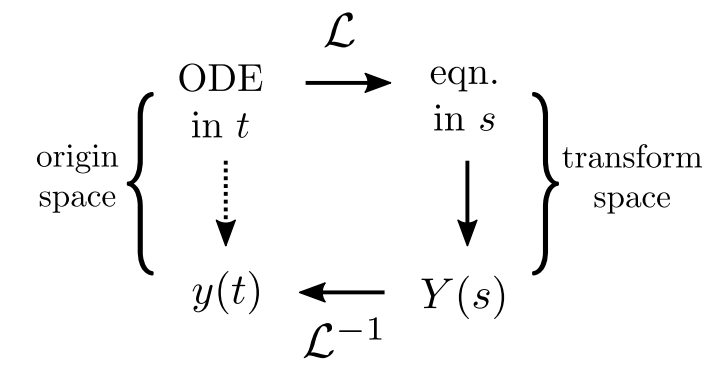
- 利用 Laplace 变换求解 ODE 过程如上图所示:
- 拉普拉斯变换将 ODE 映射到代数空间;
- 求解代数空间中的方程(组), 得到解 $Y(s)$;
- 将 $Y(s)$ 分解为容易求逆的各部件组合;
- 映射回 $y(t)$.
Example 1
方程为
$$ y'(t) = y(t). $$进行拉普拉斯变换:
$$ \underbrace{\mathcal{L}[y']}_{sY(s) - y(0)} = \underbrace{\mathcal{L}[y]}_{Y(s)} $$即
$$ (s - 1) Y = y_0 \Rightarrow Y(s) = \frac{y_0}{s - 1}. $$查表可知:
$$ \mathcal{L}[e^{at}] = \frac{1}{s - a}, $$$$ \mathcal{L}^{-1}[\frac{y_0}{s - 1}] =y_0 \mathcal{L}^{-1}[\frac{1}{s - 1}] =y_0 e^t. $$
Example 2
方程为
$$ y'' - 2 y' + y = 0, \quad Y(0) = y_0 = 1, Y'(0) = y_0' = 0. $$进行拉普拉斯变换:
$$ \underbrace{\mathcal{L}[y'']}_{s^2 Y(s) - s y(0) - y'(0)} - 2 \underbrace{\mathcal{L}[y']}_{sY(s) - y(0)} + \underbrace{\mathcal{L}[y]}_{Y(s)} = 0. $$即
$$ (s^2 - 2s + 1) Y - (s + 2)y_0 - y_0' = 0 \Rightarrow Y(s) = \frac{s + 2}{s^2 - 2s + 1} = \frac{s + 2}{(s - 1)^2}. $$分解为容易求逆的形式:
$$ Y(s) = \frac{s - 2}{(s - 1)^2} = \frac{1}{s - 1} - \frac{1}{(s - 1)^2}. $$注意到,
$$ \frac{ \mathrm{d} }{\mathrm{d}s} \left(\frac{1}{s - 1}\right) = -\frac{1}{(s - 1)^2}. $$根据 $F^{(1)}(s) = \mathcal{L}[-t f(t)]$ 以及 $\mathcal{L}^{-1}[1 / (s - 1)] = e^{t}$ 可得
$$ \mathcal{L}^{-1}[-1 / (s - 1)^2] = -te^t. $$因此方程的解为
$$ y(t) = (1 - t)e^t. $$
Example 3
方程为
$$ y'' + y = \sin \omega t, \quad y(0) = y_0 = 0, y'(0) = y_0' = 1, \quad \omega \not= \pm 1. $$进行拉普拉斯变换:
$$ \underbrace{\mathcal{L}[y'']}_{s^2 Y(s) - sy(0) - y'(0)} +\underbrace{\mathcal{L}[y]}_{Y(s)} =\underbrace{\mathcal{L}[\sin \omega t]}_{\frac{\omega}{s^2 + \omega^2}}. $$即
$$ (s^2 + 1) Y - sy_0 - y_0' = \frac{\omega}{s^2 + \omega^2}. \Rightarrow Y = \frac{1}{s^2 + 1} + \frac{\omega}{(s^2 + 1)(s^2 + \omega^2)}. $$分解为容易求逆的形式:
$$ Y = \frac{1}{s^2 + 1} + \frac{\omega}{\omega^2 - 1} \left ( \frac{1}{s^2 + 1} - \frac{1}{s^2 + \omega^2} \right ). $$查表可得
$$ \mathcal{L}[\sin \omega t] = \frac{\omega}{s^2 + \omega^2}, $$因此
$$ y(t) = \frac{\omega^2 + \omega - 1}{\omega^2 - 1} \sin t - \frac{1}{\omega^2 - 1} \sin \omega t. $$
有趣的拓展: Transfer Function
对于微分方程:
$$ \tag{O1} \sum_{k=0}^m a_k y^{(k)}(t) = \sum_{k=0}^n b_k u^{(k)} (t), $$可以用一种等价的形式表示:
$$ \tag{O2} H_1(s) Y(s) = H_2(s) U(s). $$这里 $Y(s)$ 表示 $\mathcal{L}(y)$, $U(s) = \mathcal{L}[u]$, 而
$$ H_1(s) = \sum_{k=0}^m \alpha_k s^k, \quad H_2(s) = \sum_{k=0}^n \alpha_k s^k. $$容易发现, 和严格的 (O1) 的拉普拉斯变换相比, (O2) 少了一些’常数项’. 显然, (O1) 和 (O2) 是互相确定的.
现在假设我们有另外一个方程:
$$ \tag{O3} \sum_{k=0}^p c_k u^{(k)}(t) = \sum_{k=0}^q d_k x^{(k)} (t), $$显然它有
$$ \tag{O4} H_3(s) U(s) = H_4(s) X(s). $$现在的问题是, $y, x$ 的间的关系是否能够由
$$ \tag{O5} Y(s) =\frac{H_2(s) H_4(s)}{H_1(s) H_3(s)} X(s) $$确定?
答案是 ok 的.
假设 (O2) 和 (O4) 的完整的经过拉普拉斯变换后的方程为:
$$ H_1(s) Y(s) = H_2(s) U(s) + R_1(s), \\ H_3(s) U(s) = H_4(s) X(s) + R_2(s), \\ $$这里 $R_1, R_2$ 是和 $Y, U, X$ 无关的项. 于是, 此时我们可以得到:
$$ \tag{O6} Y(s) =\frac{H_2(s) H_4(s)}{H_1(s) H_3(s)} X(s) + \frac{1}{H_1(s)} R_1(s) + \frac{H_2(s)}{H_1(s) H_3(s)} R_2(s). $$即
$$ \tag{O7} H_1(s) H_3(s) Y(s) = H_2(s) H_4(s) X(s) + H_3(s) R_1(s) + H_2(s) R_2(s). $$既然 (O1) (O3) 共同确定的解一定是 (O6) 或者 (O7) 的解, 那它一定是由 (O5) 所确定的方程的解.
换言之, 我们可以不必在意一些’常数项’ $R_1, R_2$, 通过拉普拉斯变换和代数操作方便地进行变量替换.
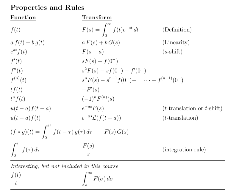
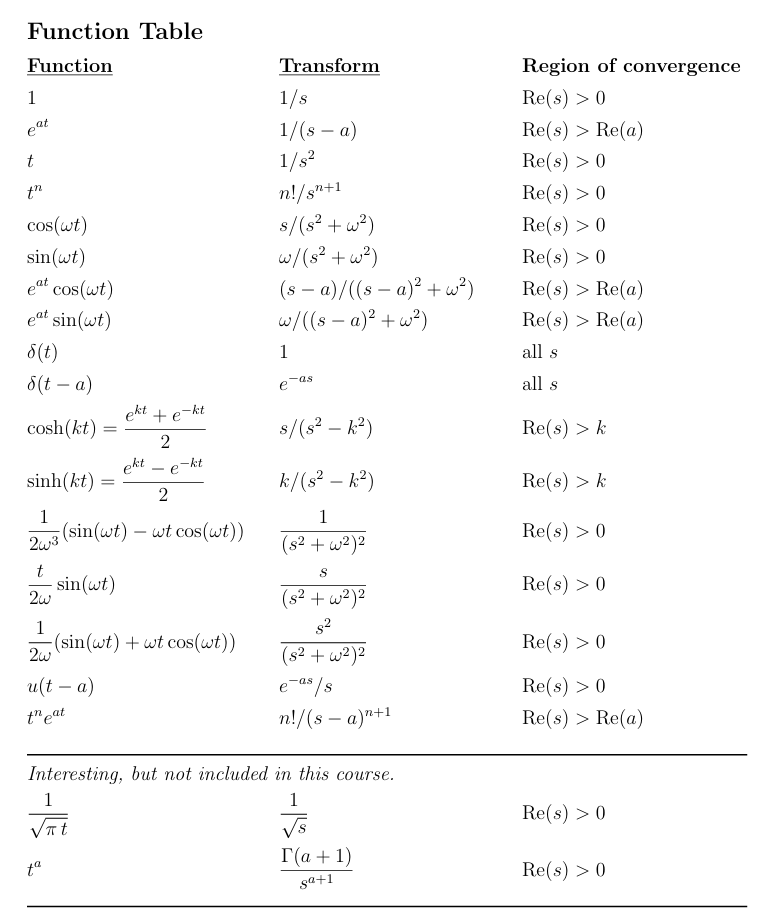
常见的 Laplace 变换