Product Quantization for Nearest Neighbor Search
预备知识
(Nearest Neighbor Search) 在一个大小为 $n$ 的集合 $\mathcal{Y} \subset \mathbb{R}^D$ 中找到和 query $x \in \mathbb{R}^D$ 最近的向量:
$$ \text{NN}(x) = \underset{{y \in \mathcal{Y}}}{\text{argmin}} \: d(x, y). $$这个匹配的时间复杂度一般是 $\mathcal{O}(nD)$, 显然当向量数据库很大的时候, 开销是难以接受的.
(Approximate Nearest Neighbor (ANN) Search) ANN 希望将精确匹配弱化为高概率匹配, 以避免反复的相似度计算过程. 比如大名鼎鼎的局部敏哈希 (Locality-Sensitive Hashing) 通过哈希来实现这一目的, 其目标是:
- 相似的数据点 → 高概率哈希到同一桶.
- 不相似的数据点 → 低概率哈希到同一桶.
(Vector Quantization) 给定 Codebook $\mathcal{C} = \{c_i \in \mathbb{R}^D: i =0,1,\ldots, k - 1\}$, quantizer $q(\cdot)$ 定义为
$$ q(x) = \underset{c_i \in \mathcal{C}}{\text{argmin}} \: d(x, c_i). $$当 $k=256$ 时, 可以认为整个向量数据库可以被压缩为 8-bit integers 表示. 对于以 $c_i$ 为中心的向量 $\mathcal{V}_i := \{x: q(x) = c_i\}$ (这个集合可以作为一个 Voronoi cell), 均可以用 $c_i$ 近似表达. 当然这里面有一定的误差.
核心思想
虽然 ANN 已经能够很好地解决 Search 过程中高昂的时间复杂度 (以一定的误差为代价), 但是过往的方法往往只是考虑 Time & Precision 的平衡, 忽略了存储上的问题. 当向量数据库增大到亿级别的时候, 这个问题是不得不重视的.
因此, 本文希望将向量通过向量量化后存储起来, 减少 Memory 占用的同时方便 Search.
(Product Quantization) 在普通的向量量化基础上, PQ 将整个向量均匀分成 $m$ 段 ($D$ 可以被 $m$ 整除) 然后分别进行向量量化:
$$ \underbrace{ x_1, x_2, \ldots, x_{D/m} }_{u_1} \underbrace{ x_{D/m + 1}, x_{D/ m + 2}, \ldots, x_{2D/m} }_{u_2} \ldots, \underbrace{ x_{D - D/m + 1}, x_{D - D/ m + 2}, \ldots, x_{D} }_{u_m} \\ \longrightarrow \left[ q_1\left( u_1(x) \right), q_2\left( u_2(x) \right), \ldots, q_m\left( u_m(x) \right) \right]. $$假如每个 Codebook $\mathcal{C}_i$ 的 size 均为 $k$, 则总共有 $k^m$ 个中心和 $\mathcal{V}_i$.
(Tips:) 为了保证每个分段的能量的均衡 (相似的 magnitude), 作者提到可以用随机正交矩阵来调节. 但是作者不建议这么做: 作者认为一般来说元素的分布也是有信息的, 最好还是遵循原本的.
(Search with Quantization) 在向量量化的基础上进行匹配有方式:
Symmetric distance computation (SDC): 即无论是 query $x$ 还是数据库中的 $y$ 都用其量化后的结果进行匹配:
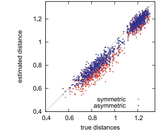
$$ \hat{d}(x, y) = d(q(x), q(y)) = \sqrt{ \sum_{j=1}^m d(q_j(x), q_j(y)) }. $$Asymmetric distance computation (ADC): 仅数据库中的 $y$ 用其量化后的结果进行匹配:
$$ \hat{d}(x, y) = d(x, q(y)) = \sqrt{ \sum_{j=1}^m d(x, q_j(y)) }. $$显然 ADC 比 SDC 在精度方面更有优势, 且时间复杂度上几乎没有差别 (如下图所示).
FAISS
- 下面是 FAISS 官方给的构建向量数据库以及 Search 的例子. 第三部分便是应用了本文所提出的方案.
# %%

import numpy as np
import faiss

# %%

d = 64                           # dimension
nb = 100000                      # database size
nq = 10000                       # nb of queries
np.random.seed(1234)             # make reproducible
xb = np.random.random((nb, d)).astype('float32')
xb[:, 0] += np.arange(nb) / 1000.
xq = np.random.random((nq, d)).astype('float32')
xq[:, 0] += np.arange(nq) / 1000.

xb[:5], xq[:5]
# %%

# 一般的精确搜索, O(nD) 复杂度
# k: 返回最近的 k 个 neighbors

index = faiss.IndexFlatL2(d)   # build the index
print(index.is_trained)
index.add(xb)                  # add vectors to the index
print(index.ntotal)

k = 4                          # we want to see 4 nearest neighbors
D, I = index.search(xb[:5], k) # sanity check
print(I)
print(D)                       # the first columns are zero
D, I = index.search(xq, k)     # actual search
print(I[:5])                   # neighbors of the 5 first queries
print(I[-5:])                  # neighbors of the 5 last queries

# True
# 100000
# [[  0 393 363  78]
#  [  1 555 277 364]
#  [  2 304 101  13]
#  [  3 173  18 182]
#  [  4 288 370 531]]
# [[0.        7.1751733 7.2076297 7.2511625]
#  [0.        6.3235645 6.684581  6.799946 ]
#  [0.        5.7964087 6.391736  7.2815123]
#  [0.        7.2779055 7.5279875 7.662846 ]
#  [0.        6.7638035 7.2951202 7.368815 ]]
# [[ 381  207  210  477]
#  [ 526  911  142   72]
#  [ 838  527 1290  425]
#  [ 196  184  164  359]
#  [ 526  377  120  425]]
# [[ 9900 10500  9309  9831]
#  [11055 10895 10812 11321]
#  [11353 11103 10164  9787]
#  [10571 10664 10632  9638]
#  [ 9628  9554 10036  9582]]

# %%

# 通过向量量化得到 Voronoi cells
# 1. 通过 cell 的中心进行初筛
# 2. 在候选的 cells 中进行精确匹配
# nlist: number of cells
# nprobe: the number of cells that are visited to perform a search

nlist = 100
k = 4
quantizer = faiss.IndexFlatL2(d)  # the other index
index = faiss.IndexIVFFlat(quantizer, d, nlist)
assert not index.is_trained
index.train(xb)
assert index.is_trained

index.add(xb)                  # add may be a bit slower as well
D, I = index.search(xq, k)     # actual search
print(I[-5:])                  # neighbors of the 5 last queries
print(D[-5:])
index.nprobe = 10              # default nprobe is 1, try a few more
D, I = index.search(xq, k)
print(I[-5:])                  # neighbors of the 5 last queries
print(D[-5:])

# [[ 9900  9309  9810 10048]
#  [11055 10895 10812 11321]
#  [11353 10164  9787 10719]
#  [10571 10664 10632 10203]
#  [ 9628  9554  9582 10304]]
# [[6.531542  7.003928  7.1329813 7.32678  ]
#  [4.3351846 5.2369733 5.3194113 5.7031565]
#  [6.0726957 6.6140213 6.732214  6.967677 ]
#  [6.637367  6.6487756 6.8578253 7.091343 ]
#  [6.218346  6.4524803 6.581311  6.582589 ]]
# [[ 9900 10500  9309  9831]
#  [11055 10895 10812 11321]
#  [11353 11103 10164  9787]
#  [10571 10664 10632  9638]
#  [ 9628  9554 10036  9582]]
# [[6.531542  6.978715  7.003928  7.013735 ]
#  [4.3351846 5.2369733 5.3194113 5.7031565]
#  [6.0726957 6.576689  6.6140213 6.732214 ]
#  [6.637367  6.6487756 6.8578253 7.009651 ]
#  [6.218346  6.4524803 6.5487304 6.581311 ]]


# %%

# 通过 Product Quantization 进一步压缩存储占用

nlist = 100
m = 8                             # number of subquantizers
k = 4
quantizer = faiss.IndexFlatL2(d)  # this remains the same
index = faiss.IndexIVFPQ(quantizer, d, nlist, m, 8)
                                    # 8 specifies that each sub-vector is encoded as 8 bits
index.train(xb)
index.add(xb)
D, I = index.search(xb[:5], k) # sanity check
print(I)
print(D)
index.nprobe = 10              # make comparable with experiment above
D, I = index.search(xq, k)     # search
print(I[-5:])


# [[   0   78  159  424]
#  [   1  555 1063    5]
#  [   2  304  179  134]
#  [   3  182  139  265]
#  [   4  288  531   95]]
# [[1.6623363 5.9748235 6.432223  6.598652 ]
#  [1.3124933 5.700293  5.9881134 6.2415333]
#  [1.8071327 5.6087813 6.116017  6.2952175]
#  [1.7520823 6.575944  6.6075144 6.7987113]
#  [1.4028182 5.7459674 6.2515984 6.298007 ]]
# [[10437 10560  9842  9432]
#  [11373 10507  9014 10494]
#  [10719 11291 10494 11383]
#  [10630  9671 10972 10040]
#  [10304  9878  9229 10370]]